Take Home Exercise 3

Resale trends of flats in Singapore

Author

Prachi Ashani

Published

February 11, 2023

Modified

March 11, 2023

The task

For the purpose of this study, we focus on the resale of 3-ROOM, 4-ROOM and 5-ROOM types flats in Singapore. While we do explore the overall data from 2017, we mainly focus on deep diving into 2022 to gain some insights.

About the data

The data is covers details of different types of houses sold in Singapore from January 2017 to February 2023. The data is sourced from data.gov.sg.

The dataset contains the following fields:

Field name	Field type	Description
month	date (yyyy-mm)	The year and month in which the property resale is recorded
town	character	The planning area in which the property sale is recorded
flat_type	character	The type of flat that is sold
block	numeric	The block number of the property sold
storey_range	categorical	Captures the storey in range of the property sold
floor_area_sqm	numeric	The floor size of the property sold in square meters
flat_model	character	The model of the flat sold
lease_commence_date	numeric (yyyy)	The year in which the lease of the property commenced
remaining_lease	character (years, months)	The time remaining for expiration of the property lease
resale_price	numeric	The price at which the property is sold

Installing the packages

We install the required R packages to perform the analysis.

pacman::p_load(ggstatsplot, readxl, performance, parameters, see, FunnelPlotR, plotly, knitr, crosstalk, DT, ggdist, gganimate, ggpubr, hrbrthemes, ggridges, ggiraph, viridis, patchwork, scales, treemap, testthat, Hmisc, tidyverse)

Importing the data

resale <- read_csv("data/resale_flat prices.csv")

Rows: 129909 Columns: 11
── Column specification ────────────────────────────────────────────────────────
Delimiter: ","
chr (8): month, town, flat_type, block, street_name, storey_range, flat_mode...
dbl (3): floor_area_sqm, lease_commence_date, resale_price

ℹ Use `spec()` to retrieve the full column specification for this data.
ℹ Specify the column types or set `show_col_types = FALSE` to quiet this message.

Data Wrangling and Preparation

Preparing the data

For the purpose of our analysis, we need to wrangle the data - create new variables, split fields to get more meaningful insights, and convert variables to the right datatype. Additionally, for overall analysis, we limit our dataset to 3-room, 4-room, and 5-room flat types from 2017 to 2022. This will help us compare year-on-year.

Creating new variables age, price per square meter (psm), and price in thousands (kprice).

resale <- resale %>%
  mutate(psm = round(resale_price / floor_area_sqm)) %>% 
  mutate(kprice = round(resale_price / 1000)) %>% 
  mutate(age = round(2022 - lease_commence_date))

Separating the month column (yyyy-mm) into year (yyyy) and month (mm).

resale <- resale %>%
  separate(month, c("year", "month"), sep = "-")

Converting the string variables to integer variables.

resale$year <- strtoi(resale$year)
resale$month <- strtoi(resale$month)

Exploring the overall data

Ridgeline plot

A Ridgeline plot (sometimes called Joyplot) shows the distribution of a numeric value for several groups.

From the plot below, we see that the resale price distribution over time for planning areas such as Toa Payoh, Bukit Timah, Kallang, Central Area, and Queenstown is wider compared to the other areas. This means the resale price range for properties here is broad.

While the resale prices years over the years, the distribution for all the areas remain somewhat consistent.

Code

ggplot(data = resale, aes(x = kprice, y = town, fill = after_stat(x))) +
  
  geom_density_ridges_gradient(scale = 3, rel_min_height = 0.01) +
  
  theme_classic2() +
    theme(
      text = element_text(family = "Georgia"),
      plot.title = element_text(face = "bold"),
      legend.position="none",
      ) +
  
  scale_fill_viridis(name = "resale_prices", option = "F") +
  
  labs(title = 'Resale Prices by Planning Area: {frame_time}', x = "Resale Prices in 000s", y = "Planning Areas") +
  
  transition_time(resale$year) +

  ease_aes('linear')

Picking joint bandwidth of 35

Boxplot

We see the price range for all three type of flats (3-room, 4-room, and 5-room) have increased over the years from 2017 to 2022. Correspondingly, the median prices of each of the flat types have also increased over the years.

Code

ggplot(data = resale, aes(x = flat_type, y = kprice, fill = flat_type)) +
  
  geom_boxplot(mapping = NULL) +
  
  theme_classic2() +
    theme(
      text = element_text(family = "Georgia"),
      plot.title = element_text(face = "bold"),
      legend.position="none",
      ) +
  
  scale_fill_viridis(option = "F", discrete = TRUE) +

  labs(title = "Resale prices in 000s by flat-type: {frame_time}", x = "Flat type", y = "Resale Prices in 000s") +
  
  transition_time(resale$year) +
   
  ease_aes('linear')

Deep Dive: 2022

We now limit our analysis to 2022. This helps us to draw better insights about the 3-room, 4-room, and 5-room flat type sale trend in Singapore.

Filtering by room-type and year.

resale_2022 <- resale %>%
  filter(year == 2022, flat_type %in% c("3 ROOM", "4 ROOM", "5 ROOM"))

Studying the data

Data Summary

From the table below, we see over 24,000 property transactions were recorded in 2022 for 3-room, 4-room, and 5-room flats in Singapore.

my_sum <- summary(resale_2022) 
knitr::kable(head(my_sum), format = 'html')

year	month	town	flat_type	block	street_name	storey_range	floor_area_sqm	flat_model	lease_commence_date	remaining_lease	resale_price	psm	kprice	age
Min. :2022	Min. : 1.000	Length:24372	Length:24372	Length:24372	Length:24372	Length:24372	Min. : 51.00	Length:24372	Min. :1967	Length:24372	Min. : 200000	Min. : 3333	Min. : 200.0	Min. : 3.00
1st Qu.:2022	1st Qu.: 3.000	Class :character	Class :character	Class :character	Class :character	Class :character	1st Qu.: 81.00	Class :character	1st Qu.:1985	Class :character	1st Qu.: 428000	1st Qu.: 4838	1st Qu.: 428.0	1st Qu.: 8.00
Median :2022	Median : 5.000	Mode :character	Mode :character	Mode :character	Mode :character	Mode :character	Median : 93.00	Mode :character	Median :1998	Mode :character	Median : 515000	Median : 5368	Median : 515.0	Median :24.00
Mean :2022	Mean : 6.047	NA	NA	NA	NA	NA	Mean : 94.08	NA	Mean :1997	NA	Mean : 536394	Mean : 5736	Mean : 536.4	Mean :24.54
3rd Qu.:2022	3rd Qu.:10.000	NA	NA	NA	NA	NA	3rd Qu.:110.00	NA	3rd Qu.:2014	NA	3rd Qu.: 610000	3rd Qu.: 6176	3rd Qu.: 610.0	3rd Qu.:37.00
Max. :2022	Max. :12.000	NA	NA	NA	NA	NA	Max. :159.00	NA	Max. :2019	NA	Max. :1418000	Max. :14731	Max. :1418.0	Max. :55.00

Histogram

We analyze the distribution and the outliers in the dataset through histograms. We see that resale price in thousands and price per square unit have a right skew.

set.seed(1234)

g_price <- gghistostats(
  data = resale_2022,
  x = kprice,
  type = "bayes",
  test.value = 60,
  xlab = "resale prices in 000s"
          ) +
  
  theme_classic2() +
    theme(
      text = element_text(family = "Georgia"),
      plot.title = element_text(face = "bold"),
      legend.position="none"
      )

g_psm <- gghistostats(
  data = resale_2022,
  x = psm,
  type = "bayes",
  test.value = 60,
  xlab = "price per sqm"
)

g_farea <- gghistostats(
  data = resale_2022,
  x = floor_area_sqm,
  type = "bayes",
  test.value = 60,
  xlab = "floor area (sqm)"
) 

g_age <- gghistostats(
  data = resale_2022,
  x = age,
  type = "bayes",
  test.value = 60,
  xlab = "property age"
)

ggarrange(g_price, g_psm, g_farea, g_age, ncol = 2, nrow = 2)

Warning in grid.Call(C_stringMetric, as.graphicsAnnot(x$label)): font family
'Georgia' not found in PostScript font database

Warning in grid.Call(C_stringMetric, as.graphicsAnnot(x$label)): font family
'Georgia' not found in PostScript font database

Warning in grid.Call(C_stringMetric, as.graphicsAnnot(x$label)): font family
'Georgia' not found in PostScript font database

Warning in grid.Call(C_stringMetric, as.graphicsAnnot(x$label)): font family
'Georgia' not found in PostScript font database

Warning in grid.Call(C_stringMetric, as.graphicsAnnot(x$label)): font family
'Georgia' not found in PostScript font database

Warning in grid.Call(C_stringMetric, as.graphicsAnnot(x$label)): font family
'Georgia' not found in PostScript font database

Warning in grid.Call(C_stringMetric, as.graphicsAnnot(x$label)): font family
'Georgia' not found in PostScript font database

Warning in grid.Call(C_stringMetric, as.graphicsAnnot(x$label)): font family
'Georgia' not found in PostScript font database

Warning in grid.Call(C_stringMetric, as.graphicsAnnot(x$label)): font family
'Georgia' not found in PostScript font database

Warning in grid.Call(C_stringMetric, as.graphicsAnnot(x$label)): font family
'Georgia' not found in PostScript font database

Warning in grid.Call(C_stringMetric, as.graphicsAnnot(x$label)): font family
'Georgia' not found in PostScript font database

Warning in grid.Call(C_stringMetric, as.graphicsAnnot(x$label)): font family
'Georgia' not found in PostScript font database

Warning in grid.Call(C_stringMetric, as.graphicsAnnot(x$label)): font family
'Georgia' not found in PostScript font database

Warning in grid.Call(C_stringMetric, as.graphicsAnnot(x$label)): font family
'Georgia' not found in PostScript font database

Warning in grid.Call(C_stringMetric, as.graphicsAnnot(x$label)): font family
'Georgia' not found in PostScript font database

Warning in grid.Call(C_stringMetric, as.graphicsAnnot(x$label)): font family
'Georgia' not found in PostScript font database

Warning in grid.Call(C_stringMetric, as.graphicsAnnot(x$label)): font family
'Georgia' not found in PostScript font database

Warning in grid.Call(C_stringMetric, as.graphicsAnnot(x$label)): font family
'Georgia' not found in PostScript font database

Warning in grid.Call(C_stringMetric, as.graphicsAnnot(x$label)): font family
'Georgia' not found in PostScript font database

Warning in grid.Call(C_stringMetric, as.graphicsAnnot(x$label)): font family
'Georgia' not found in PostScript font database

Warning in grid.Call(C_stringMetric, as.graphicsAnnot(x$label)): font family
'Georgia' not found in PostScript font database

Warning in grid.Call(C_stringMetric, as.graphicsAnnot(x$label)): font family
'Georgia' not found in PostScript font database

Warning in grid.Call(C_stringMetric, as.graphicsAnnot(x$label)): font family
'Georgia' not found in PostScript font database

Warning in grid.Call(C_stringMetric, as.graphicsAnnot(x$label)): font family
'Georgia' not found in PostScript font database

Warning in grid.Call(C_stringMetric, as.graphicsAnnot(x$label)): font family
'Georgia' not found in PostScript font database

Warning in grid.Call(C_stringMetric, as.graphicsAnnot(x$label)): font family
'Georgia' not found in PostScript font database

Warning in grid.Call(C_stringMetric, as.graphicsAnnot(x$label)): font family
'Georgia' not found in PostScript font database

Warning in grid.Call(C_stringMetric, as.graphicsAnnot(x$label)): font family
'Georgia' not found in PostScript font database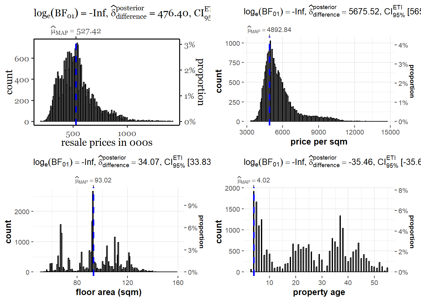

Excluding the outliers

Thus, we exclude the outliers using interquartile range for both resale price in thousands and price per square meter.

IQR_price = IQR(resale_2022$kprice)
IQR_psm = IQR(resale_2022$psm)

price_upper = quantile(resale_2022$kprice, probs = 0.75)+1.5*IQR_price
psm_upper = quantile(resale_2022$psm, probs = 0.75)+1.5*IQR_psm

We then filter out the dataset and focus on this clean data for property sales in 2022.

resale_filter <- resale_2022 %>%
  filter((resale_2022$kprice <= price_upper) & 
           (resale_2022$psm <= psm_upper))

Exploratory Data Analysis

Histogram after excluding the outliers

We see the distribution for resale price in thousands and price per square meter somewhat improve after excluding the outliers using interquartile range (IQR).

Code

m_price = mean(resale_filter$kprice)
std_price = sd(resale_filter$kprice)

dist_price <- ggplot(data = resale_filter, aes(kprice)) +
  geom_histogram(aes(y=after_stat(density)), fill = "deeppink4", color = "black") + 
  
  stat_function(fun = dnorm, args = list(mean = m_price, sd = std_price), col="darkslategray", size = .8) +
  
  theme_classic2() +
    theme(
      text = element_text(family ="Georgia"),
      plot.title = element_text(face = "bold"),
      axis.text.y = element_blank(),
      axis.title.y = element_blank(),
      axis.ticks.y = element_blank(),
      axis.line.y = element_blank(),
      ) +
  
  labs(title = 'Distribution of resale price in 000s')

Warning: Using `size` aesthetic for lines was deprecated in ggplot2 3.4.0.
ℹ Please use `linewidth` instead.

Code

m_psm = mean(resale_filter$psm)
std_psm = sd(resale_filter$psm)

dist_psm <- ggplot(data = resale_filter, aes(psm)) +
  geom_histogram(aes(y=after_stat(density)), fill = "deeppink4", color = "black") + 
  
  stat_function(fun = dnorm, args = list(mean = m_psm, sd = std_psm), col="darkslategray", size = .8) +
  
  theme_classic2() +
    theme(
      text = element_text(family ="Georgia"),
      plot.title = element_text(face = "bold"),
      axis.text.y = element_blank(),
      axis.title.y = element_blank(),
      axis.ticks.y = element_blank(),
      axis.line.y = element_blank()
      ) +
  
  labs(title = 'Distribution of resale price in 000s')

Code

dist_price + dist_psm

`stat_bin()` using `bins = 30`. Pick better value with `binwidth`.
`stat_bin()` using `bins = 30`. Pick better value with `binwidth`.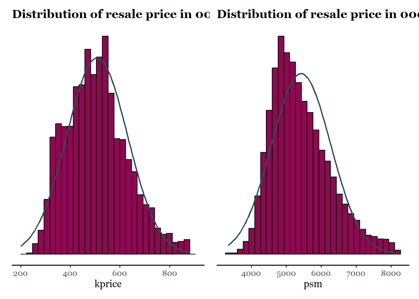

Correlation Analysis

As anticipated, the floor_area shows a strong positive correlation with resale property price.

Code

ggstatsplot::ggscatterstats(
  data = resale_filter,
  x = floor_area_sqm,
  y = kprice,
  marginal = FALSE,
  ) +

  theme_classic2() +
    theme(
      text = element_text(family ="Georgia"),
      plot.title = element_text(face = "bold")
      ) +
    
    labs(title = 'Correlation of resale price (in 000s) and floor area (sqm)', x = "Floor Area", y = "Resale Price in 000s")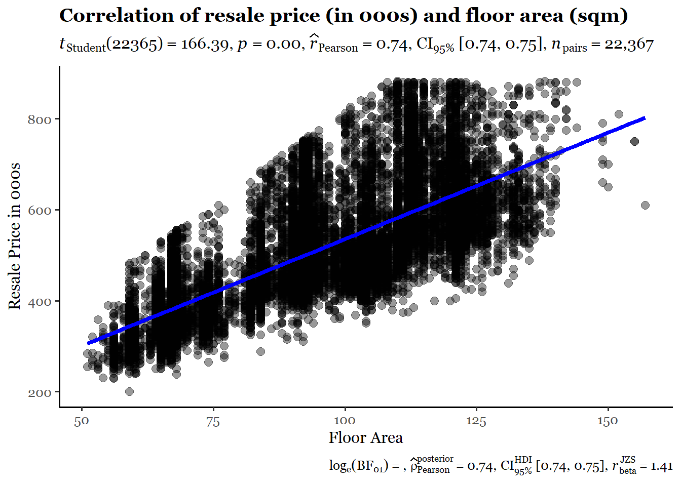

Below we see a quick snapshot of the final dataset we are going to be working with in the further analysis.

my_des <- describe(resale_filter, num.desc=c("mean","median","var","sd","valid.n"), xname = NA, horizontal=FALSE) %>% html()

Warning in png(file, width = 1 + k * w, height = h): 'width=10, height=13' are
unlikely values in pixels

my_des

resale_filter Descriptives

resale_filter

15 Variables 22367 Observations

year

n	missing	distinct	Info	Mean	Gmd
22367	0	1	0	2022	0

 Value       2022
 Frequency  22367
 Proportion     1

month

n	missing	distinct	Info	Mean	Gmd	.05	.10	.25	.50	.75	.90	.95
18300	4067	10	0.99	6.03	4.151	1	1	3	5	10	12	12

lowest : 1 2 3 4 5 , highest: 6 7 10 11 12

 Value          1     2     3     4     5     6     7    10    11    12
 Frequency   2100  1586  1895  1906  1806  1754  1963  1619  1773  1898
 Proportion 0.115 0.087 0.104 0.104 0.099 0.096 0.107 0.088 0.097 0.104

town

n	missing	distinct
22367	0	26

lowest :	ANG MO KIO	BEDOK	BISHAN	BUKIT BATOK	BUKIT MERAH
highest:	SERANGOON	TAMPINES	TOA PAYOH	WOODLANDS	YISHUN

flat_type

n	missing	distinct
22367	0	3

 Value      3 ROOM 4 ROOM 5 ROOM
 Frequency    5948  10235   6184
 Proportion  0.266  0.458  0.276

block

n	missing	distinct
22367	0	2389

lowest : 1 10 100 101 101A , highest: 989A 989C 989D 99 9A

street_name

n	missing	distinct
22367	0	540

lowest :	ADMIRALTY DR	ADMIRALTY LINK	AH HOOD RD	ALJUNIED CRES	ALJUNIED RD
highest:	YUNG AN RD	YUNG HO RD	YUNG KUANG RD	YUNG LOH RD	YUNG SHENG RD

storey_range

n	missing	distinct
22367	0	13

lowest : 01 TO 03 04 TO 06 07 TO 09 10 TO 12 13 TO 15 , highest: 25 TO 27 28 TO 30 31 TO 33 34 TO 36 37 TO 39

 Value      01 TO 03 04 TO 06 07 TO 09 10 TO 12 13 TO 15 16 TO 18 19 TO 21 22 TO 24
 Frequency      4044     5289     4904     4283     2193      974      327      192
 Proportion    0.181    0.236    0.219    0.191    0.098    0.044    0.015    0.009
                                                        
 Value      25 TO 27 28 TO 30 31 TO 33 34 TO 36 37 TO 39
 Frequency       105       26       19        7        4
 Proportion    0.005    0.001    0.001    0.000    0.000

floor_area_sqm

n	missing	distinct	Info	Mean	Gmd	.05	.10	.25	.50	.75	.90	.95
22367	0	100	0.998	94.15	22.15	65	67	76	93	110	121	123

lowest : 51 52 53 54 55 , highest: 149 150 152 155 157

flat_model

n	missing	distinct
22367	0	12

lowest :	3Gen	Adjoined flat	DBSS	Improved	Improved-Maisonette
highest:	Model A2	New Generation	Premium Apartment	Simplified	Standard

lease_commence_date

n	missing	distinct	Info	Mean	Gmd	.05	.10	.25	.50	.75	.90	.95
22367	0	53	0.999	1996	16.95	1975	1978	1984	1996	2013	2017	2018

lowest : 1967 1968 1969 1970 1971 , highest: 2015 2016 2017 2018 2019

remaining_lease

n	missing	distinct
22367	0	630

lowest :	43 years 01 month	43 years 02 months	43 years 03 months	43 years 04 months	43 years 05 months
highest:	95 years 04 months	95 years 05 months	95 years 06 months	95 years 07 months	95 years 08 months

resale_price

n	missing	distinct	Info	Mean	Gmd	.05	.10	.25	.50	.75	.90	.95
22367	0	1337	1	507804	137936	326000	350000	420000	500000	580000	675000	730000

lowest : 200000 228888 230000 238000 240000 , highest: 878000 878888 880000 881888 882000

psm

n	missing	distinct	Info	Mean	Gmd	.05	.10	.25	.50	.75	.90	.95
22367	0	3308	1	5422	944.8	4286	4463	4798	5269	5924	6610	7065

lowest : 3333 3344 3347 3348 3368 , highest: 8167 8169 8174 8178 8182

kprice

n	missing	distinct	Info	Mean	Gmd	.05	.10	.25	.50	.75	.90	.95
22367	0	605	1	507.8	137.9	326	350	420	500	580	675	730

lowest : 200 229 230 238 240 , highest: 875 878 879 880 882

age

n	missing	distinct	Info	Mean	Gmd	.05	.10	.25	.50	.75	.90	.95
22367	0	53	0.999	25.69	16.95	4	5	9	26	38	44	47

lowest : 3 4 5 6 7 , highest: 51 52 53 54 55

Violin Plots

We see the resale price distribution by flat_type (3-room, 4-room, and 5-room) using a violin plot. As expected, the median resale prices of 3-room flat type is lower than that of 4-room and 5-room. However, based on the shape of the data, we see that the resale prices of the smaller flats are more concentrated around the median than the bigger sized flats.

For price per square meter, the distribution shape for 3-room, 4-room, and 5-room is more or less similar. The price per square meter for all three room types is mostly around the median.

Violin Plot - Resale Price in 000s
Violin Plot - Price per Square Meter

Code

### Violin Plot for resale price in 000s ###

violin_kprice <- ggbetweenstats(
  data = resale_filter,
  x = flat_type, 
  y = kprice,
  type = "p",
  mean.ci = TRUE, 
  pairwise.comparisons = TRUE, 
  pairwise.display = "s",
  p.adjust.method = "fdr",
  messages = FALSE
) +
  
    theme_classic2() +
    theme(
      text = element_text(family = "Georgia"),
      
      plot.title = element_text(face = "bold"),
      
      legend.position="none",
      ) +
  
  labs(title = 'Resale Price in 000s by Flat Type - 2022', x = "Planning Area", y = "Resale Price")

violin_kprice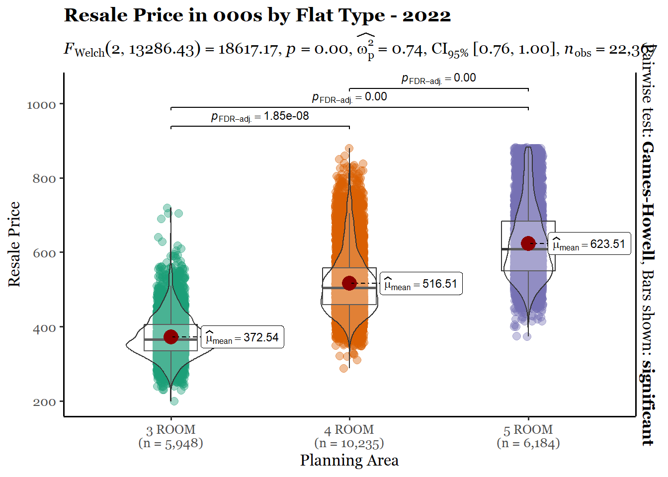

Code

### Violin Plot for resale psm in 000s ###

violin_psm <- ggbetweenstats(
  data = resale_filter,
  x = flat_type, 
  y = psm,
  type = "p",
  mean.ci = TRUE, 
  pairwise.comparisons = TRUE, 
  pairwise.display = "s",
  p.adjust.method = "fdr",
  messages = FALSE
) +

  theme_classic2() +
    theme(
      text = element_text(family = "Georgia"),
      
      plot.title = element_text(face = "bold"),
      
      legend.position="none",
      ) +
  
  labs(title = 'Price per Sqaure Meter by Flat Type - 2022', x = "Planning Area", y = "PSM")

violin_psm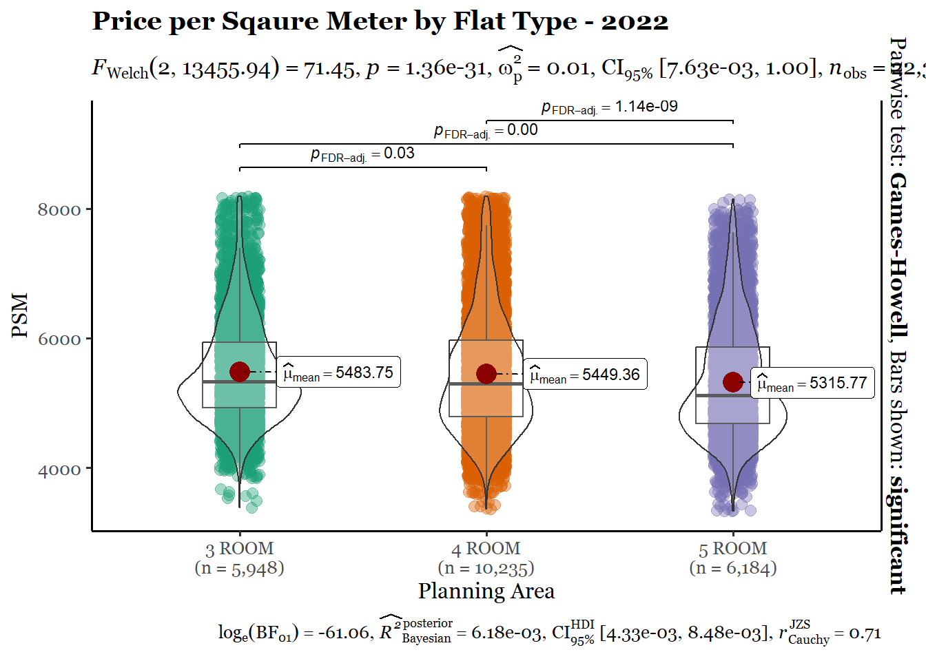

Boxplot

Next, we study the box and whiskers plot of 3-room, 4-room, and 5-room flat types across the planning regions.

We see that areas such as Jurong West and Tampines have the widest price band for 5-room type flats, especially towards the upper-side of the price. In Marine Parade, the 5-room flat types were significantly higher priced than 3-room and 4-room type flats. The opposite was true for areas such as Sembawang.

Code

p <- ggplot(data = resale_filter, mapping = aes(x = town, y = kprice)) +
  
  geom_boxplot(aes(fill = as.factor(flat_type))) +
  
  theme_classic2() +
    theme(
      text = element_text(family = "Georgia"),
      plot.title = element_text(face = "bold", size = 16),
  
      axis.text.x = element_text(angle = 90),

      ) +
  
  scale_fill_viridis(name = "resale_prices", option = "F", discrete = TRUE) +
  
  labs(title = 'Resale prices in 000s by Flat Type and Planning Area - 2022', x = "Planning Area", y = "Resale price", fill = "flat_type")

ggplotly(p)

Proportions Charts

From the donut chart, we see that the resale of 4-room properties accounted for the highest share among the three, while sale of number of 3-room and 5-room properties were similar.

From the grouped bar charts, we see that the number of 3-room type property sold is higher than the other from planning areas such as Ang Mio Ko, Bedok, and Queenstown; this is contrast to higher number of 4-room and 5-room type properties sold in areas such as Punggol, Sembawang, Senkang, etc.

Flat type proportion - overall
Flat type proportion by planning areas

Code

ft_only <- resale_filter %>%
  group_by(flat_type) %>%
  summarize(ft_count = n())%>%
  mutate(ft_pct = percent(ft_count/sum(ft_count)))

ggplot(data = ft_only, aes(x = 2, y=ft_count, fill = flat_type)) +
  geom_bar(stat = "identity") +
  coord_polar(theta = "y", start = 0) +
  xlim(c(0.5, 2.5)) +
  
  geom_text(color = "grey", size = 4, aes(y = ft_count/3 + c(0, cumsum(ft_count)[-length(ft_count)]), label = ft_pct)) +
  
  theme_classic2() +
    theme(
      text = element_text(family = "Georgia"),
      plot.title = element_text(face = "bold"),
      
      axis.line.x = element_blank(),
      axis.line.y = element_blank(),
      axis.ticks = element_blank(),
      axis.text = element_blank(),
      axis.title = element_blank(),
    
      legend.key.size = unit(5, "mm"),
      legend.position = "bottom"
      
      ) +
  
  scale_fill_viridis(option = "F", discrete = TRUE) +
  
  labs(title = 'Resale of Flats by Type and Planning Area - 2022', x = "Planning Area", y = "Flat type", fill = "Flat type")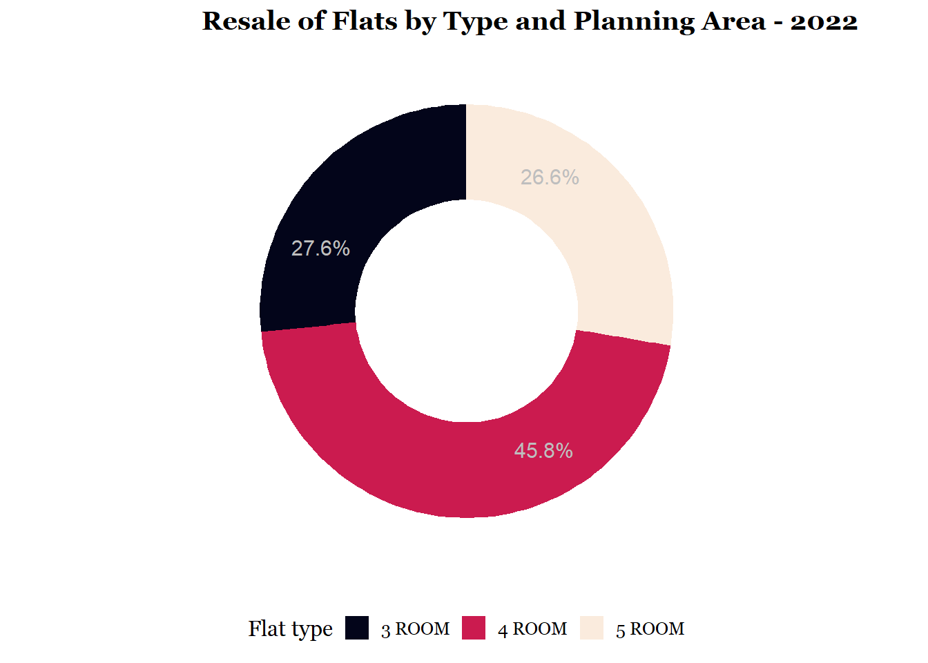

Code

p <- ggplot(data = resale_filter, aes(x = town, fill=flat_type)) +
  
  geom_bar(position = "dodge") +
  
  theme_classic2() +
    theme(
      text = element_text(family = "Georgia"),
      plot.title = element_text(face = "bold"),
      
      axis.text.x = element_text(angle = 90),
    
      legend.key.size = unit(5, "mm"),
      legend.position = "bottom"
      
      ) +
  
  scale_fill_viridis(option = "F", discrete = TRUE) +
  
  labs(title = 'Resale of Flats by Type and Planning Area - 2022', x = "Planning Area", y = "Flat type", fill = "Flat type")

ggplotly(p)

Treemap

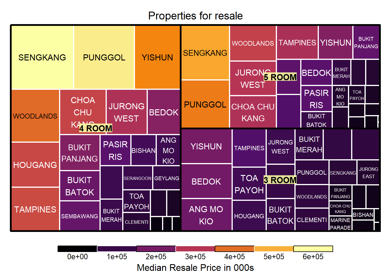
Through the treemap, we see on overall glimpse of flat types by prices per square meter and resale prices in 000s across all planning areas.

treemap (resale_filter,
              index= c("flat_type", "town"),
              vSize= "psm",
              vColor = "kprice",
              type= "manual",
              palette = inferno(5),
              force.print.labels = F,
              border.col = c("black", "white"),
              border.lwds = c(3,2),
              title= "Properties for resale",
              title.legend = "Median Resale Price in 000s"
              )

References

Ridgeline Plot, From Data to Viz, accessed 15 February 2023
Joel Carron, Violin Plots 101: Visualizing Distribution and Probability Density, Mode, 13 December 2021
Simon Foo, Analysis of Singapore’s Private Housing Property Market Prices (July 2017 to 2022), RPubs, 21 July 2022
Kenneth Low, Analysis of property market in Singapore, RPubs, accessed 15 February 2023
Wang Wenyi, An analysis of Singapore property resale market price based on transaction from 2017 to 2019, RPubs, 17 July 2020
Isabelle Liew, HDB resale prices rise 2.3% in Q4, slowest increase in 2022, The Straits Times, 01 February 2023